
By: Jeremy Parker Yang and Harmon Bhasin
General problem Overview
An important area of analysis in scRNA-seq is comparing the transcriptomic profiles of cells from two biological states. The most common approaches utilize clustering of all cells in both samples followed by downstream analysis measuring differential abundance. The issue with predefined clustering (unsupervised learning approach) is that differential abundance (DA) subpopulations may not align with a clear cluster structure based on cell type/sample. In addition, these clusters do not take into account the biological state of each cell. This leads to cell subpopulations that may not be representative of the differences between biological states.
This motivated the authors to take a supervised approach to clustering. An earlier work that utilized multiple local two-sample tests for hyperspheres centered at randomly selected cells failed to accurately delineate DA subpopulations. Seeing this gap in the literature, the authors introduced differential abundance sequencing (DA-seq), a supervised approach that utilizes the biological state of each cell to identify and delineate the cell subpopulations most representative of the differences between two biological states. The key difference between this approach and those most commonly used is that they focus on individual cells instead of predefined clusters.
Brief description of method
In conventional DA analysis, clustering is done on cells in both biological states. These clusters are then analyzed for DA states. DA-seq takes a different approach where it does not use initial clusters, but instead measures the abundance of a state per cell using its neighbors. Clustering then is done on cells with differential abundance. This process is done in four steps:
Step 1) Calculate multiscale cell score from kNN
- Instead of a DA measure at the cluster level, we want to assign each cell with its own DA measure. This cell score is based on the cell’s k nearest neighbors. The score is multiscale in that different values of k are used to increase the quality of our DA estimation (since areas will vary in density and having k values that are too high or too low might lead to under or overfitting of the data) and resolve issues of choosing an optimal k value. Each score with value k represents an estimate of the DA measure at a different scale.
- Each cell x_i gets a score vector where each element is a score for a different value k
- The score is given by
- Where g is the probability of the cell being in a state divided by the percent of cells in that state
- N_1(xi;k)/k estimates the probability of a point being labeled as state 1
- n_1/n estimates the probability of sampling state 1
Step 2) Calculate the DA measure utilizing a logistic regression classifier
- In the previous step, we get multiscale score vectors for each cell. We want to map this to a single number to represent the DA measure. It’s safe to assume that cells in DA subpopulations whose neighborhoods are enriched with cells from one biological state tend to be closer to each other in the l-dimensional score than other cells. Hence, we can use a logistic regression classifier that is trained to predict the state of a cell given its multiscale score vectors. L2 regularization is used to ensure that the output is smooth, and the DA measures across cells are localized.
- The regularization hyperparameter lambda is fit using cross validation
- The output of the logistic regression classifier estimates the posterior phat_i = Pr(y_i=1 | x_i)
- Finally, the DA measure is
3) Cluster on DA cells only using SNN + Louvian
- Now that each cell has a DA score, we want to find clusters of DA cells
- Cells are considered DA if their DA metric is above the threshold τh or below the threshold τl. A permutation test is used to determine which threshold values are DA.
- In this test, the null distribution is created by calculating the DA score (step 1 and 2) for each cell and randomly permuting its state.
- The Seurat pipeline is utilized for clustering. First, a shared nearest neighbor (SNN) graph is generated using euclidean distance on the original dimensionality reduced gene space. This graph is made with all cells, including cells that are not DA. Second, non DA cells are removed from the SNN graph. Third, a modularity based clustering algorithm clusters the DA cells (Louvian).
- These clusters represent DA subpopulations
4) Select features for DE using STG optimization
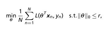
- We want to identify characteristic genes for each DA subpopulation. This can be done with standard differential expression analysis techniques. The authors propose their own method, framing this as a feature selection problem by identifying the smallest set of genes that distinguish a DA subpopulation. They select features using empirical risk minimization with an l_0 constraint.
- STG introduces a nonconvex relaxation of the optimization problem where each STG is a relaxed Bernoulli variable. Hence they’re able to reformulate their ERM problem into a risk minimization problem where they’re able to optimize by gating the variable x and minimize the number of expected active gates. This gives them a solution solved via gradient descent, where lambda is a regularized parameter that can be optimized.
- Formulate feature selection as empirical risk minimization (ERM)
- where r is the number of selected features, L is the loss function, and theta are the parameters of a linear model or more complex neural network
- Introduce STG (Stochastic Gate) approach to nn, which provides a nonconvex relaxation of the optimization in the equation above.
- Each STG is a relaxed Bernoulli variable zd, where P(zd = 1) = πd, d = 1, . . . , D, and D is the number of genes after an initial screening to remove genes with low expression.
How was the method evaluated?
This method was evaluated using four real datasets including (a) severe versus mild COVID-19 patients, (b) melanoma patients with immune checkpoint therapy responders versus non-responders, (c) embryonic development at two time-points, and (d) young versus aged brain tissue, along with two simulated datasets.
DA subpopulation analysis successfully identified COVID-19 severity markers in different cell types, such as nonresident macrophages (nrMa) and cytotoxic T cells (CTL), from the comparison of scRNA-seq nasopharyngeal/pharyngeal swab samples between mild and severe COVID-19 patients.
Similarly, comparing two types of melanoma patients, including those responding to immune checkpoint therapy and those not, a total of 70% of cells from scRNA-seq dataset are detected with a significant DA measure.
On the other hand, dermal cell differentiation patterns during embryonic development of mouse had been successfully identified using DA-seq method.
During comparison between scRNA-seq datasets of young versus aged brain tissues collected from mice, no DA subpopulation was identified as per the expectation.
The simulated datasets consisted of scRNA-seq data from a previous paper, and a perturbed Gaussian Mixture Model (GMM). In both simulated datasets, DA-seq successfully extracts the artificial DA subpopulations and outperforms similar clustering techniques like Cydar.
What novel insights were obtained using this method?
This approach allows us to identify regions with differential abundance between two states. In general, compared to methods that cluster the data initially, DA-seq identifies subpopulations with higher DA levels. DA seq not only recovered results that were similar to standard approaches, but also revealed striking unreported DA subpopulations, which informs on cellular functions, known and unknown genes, and greatly increases the resolution of cell type identity in different clinical states of disease. Allows us to use cells generated in a single scRNA-seq experiment and compare cells conditioned on the expression status of a single marker. You don’t need to cluster to figure out DA. Using an STG approach to optimization allows you to better select features.
What are the strengths and weaknesses of this method?
Strengths
- detecting salient DA subpopulations not confined to any predefined cluster,
- no prior knowledge required for differentiation of specific cells, and
- the use of an STG provides a prediction score as a linear combination of its selected genes that best separate each DA subpopulation from the rest of the cells
Weaknesses
- reliance on large sample sizes and model validation which could lead to overfitting in regions with low data density,
- lack of causal inference technique for gene selection, lack of batch effect removal, and
- the use of kNN on all cells which may be a computational bottleneck for very large datasets.
