As it is built on top of Java, Processing is capable of object-oriented programming. The notion of objects and how they make our code more modular and easy to read was the main take-away from Chapters 7 and 8 of “Learning Processing”.

So what are objects? They describe an instance of a ‘class’ which has properties and capabilities embedded into it. The idea is to write our code with a class containing variables as its properties and functions as its capabilities and later declare instances of that class as the objects in our composition. Writing code in a object-oriented approach will become very useful when we want to have dozens or hundreds of “things” in our viewport behaving a certain way, like we will have happening when we start coding particle systems and autonomous agents. But we first need to learn abt arrays and arraylists which we haven’t covered yet.

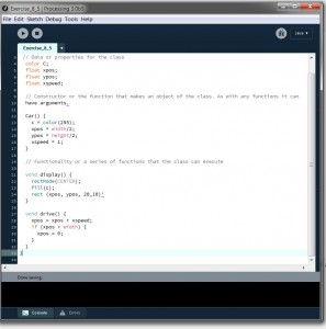
Writing a class is pretty straightforward. Each class contains four elements: name, data, constructor, and methods.

Writing a Class

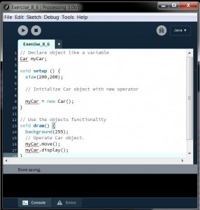
In order to use the class, you must first declare the object(s) as you would declare a global variable. In the case of an object, the type is the name class and the variable name is the name of the object.

Then you need to initialize them in the setup() function. Lastly you invoke the objects’ functionality by using dot syntax notation in the draw() function.

Using a class

Now on to this week’s project. I decided to do two compositions. The first one is simply code refactoring per Lesson 3 guidelines. I reorganized my previous composition using object-oriented programming and it allowed me to reuse my class twice creating a more interesting pattern. I also added a line of code to make the coloring of the pattern dynamic and display the colors of a rainbow by using sines and cosines in each of RGB parameters. The first composition can be found here.

The second compostion, Sines and Cosines, is the more interesting one. It is still a work in progress. But my idea was to mess around with the sines and cosines functions. As these functions are periodic, they are well behaved and the range of values is well controlled. I also had to reach out and learn a little bit of transformations and frameCount, a key component in making the drawing dynamic. In this composition, I needed to find a way to move the drawing center from the upper left corner to the middle of the screen and translate() allows that. By using frameCount inside the sines and cosines functions, you make the these functions oscillate for each loop cycle so the values keep changing and the drawing becomes dynamic. The same technique was applied to the fill() in the first composition so that the colors change for each loop cycle. Compositions like this could very well be the starting point for a building design. There is a way to export the lines into Rhino and I have to look into that. mouseX and mouseY were used to change where the second point of the lines is drawn but it doesn’t really behave as smoothly as I’d like. The composition can be found here.

See you next week!