ClusterVisualization

Link

The last couple of weeks I have been working on visualizing CONDOR cluster data in our system, that is either the CAVE, the devlab etc.

Currently, the output looks something like this:

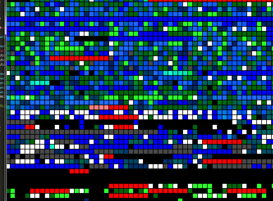
Current cluster monitor.

Each single cell represents a slot which can run an assigned job. Multiple slots are part of a node (a single computer) and multiple nodes are formed into groups. The coloring depicts the load from blue (low load = bad) to green (high load = good, efficient). Red nodes show offline nodes, black ones have missing information and grey ones are occupied otherwise. This display is updated every 20 minutes.

The approach I took was separating everything into their hierarchical structure: slots into nodes into groups:

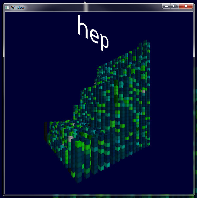
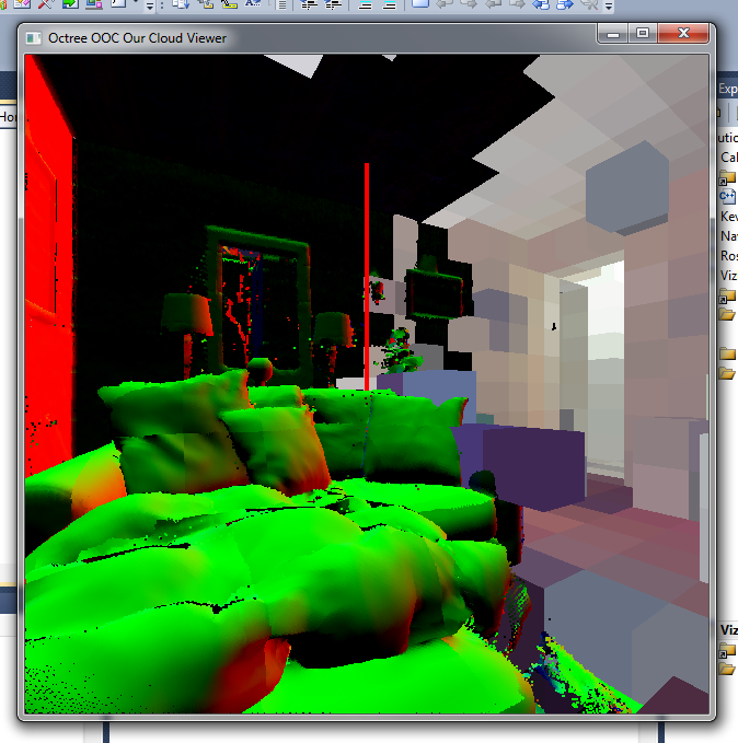
The high-energy physics group

This is the high-energy group. Many computers and you can tell at a glance that these computers are quite powerful, as they stack really high. Most of them are running jobs at different efficiency.

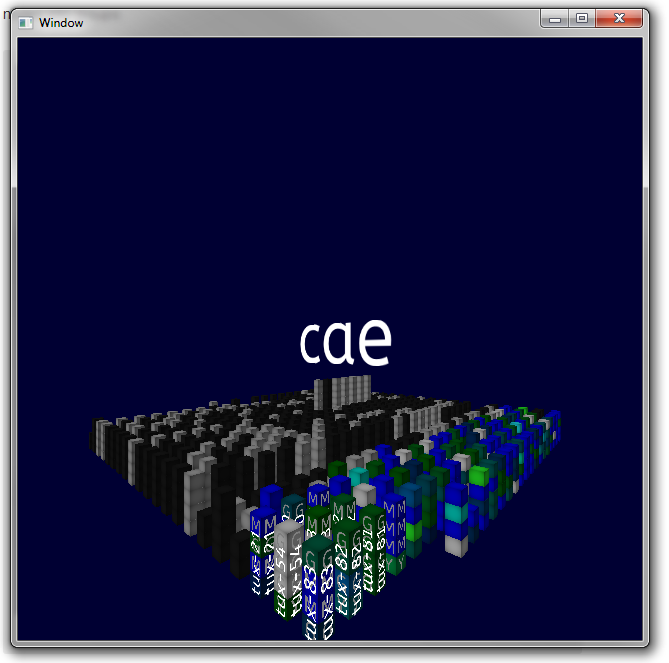
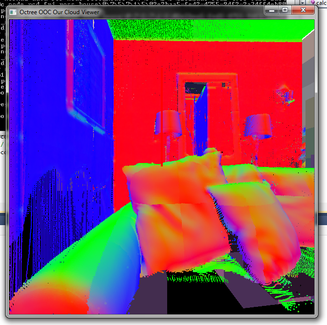
The cae group

The cae pool, on the other hand, looks completely different. Many low-powered computers with 4-8 cores, which are also not accessible (grey or black). If you move closer to the nodes, a single letter per slot shows you which job group this job belongs to. Many jobs are recurrent and therefore have their own letter (for example, Y or G). Overlaid in white is the short node name.

The cluster in action

The best thing is that we have multiple log files and we can cycle through them. Not only can you see how jobs move through the cluster and load changes, but also how the groups grow and shrink if new computers join the group or are going offline.

There are also two main data highlights in here the load view, as above, and the job view, in which the same job class is highlighted throughout the system.

Seeing this visualization in the CAVE is very interesting as you are surrounded by these massive towers. The CHTC group liked it very much so far and we will demo this system next week during CONDOR week 2014.

High Resolution Scans

Posted on April 4, 2014 by mbroecker

I scanned the concrete pillar in my office to see if we get resolution high enough to investigate small details — in this case the air bubbles and enclosures in the concrete, in the proposed project bullet holes and dents.

The distance between scanner and surface was about 1 foot and only a single scan was taken. In the scanner software I selected a small window. Unfortunately, the scanner does not tell which coordinate system this is based on, so I had to eyeball it. For further reference, this is how I think it looks:

Scanner coordinate system.

The scanning was set to the highest resolution and quality (4x supersampling?) settings and took about an hour — this is really only practical if we want to scan such a small area. Imported into SCENE, it shows up as about a one square-foot area containing about 24 million points:

High resolution scan in SCENE.

The scan dataset is about 700MB in size. We get a theoretical resolution of 24M/(400*400)mm2 = 150 pts/mm2. That seems rather high. Note that with multiple scans and interleaved scan points this number would increase further.

On a similar note, SCENE breaks down at these small scales (I think it’s more designed for surveying) and has problems displaying them, even after setting the near plane to 0.01. Movement is also way too coarse to be useful at these small scales. This is as close as we can go:

Scene close up (looks like the moon surface)

The next steps will be exporting this data and displaying it with our software. Maybe it will be useful starting a small PCL close-up viewer, as the current octree generation is between 0.25m and 0.3m and would therefore put all points in a single voxel. An alternative could be increasing the scale of the scan data and multiplying the coordinates of all points by a fixed scale, eg. 100. That could create an octree hierarchy and we could use our out-of-core viewer for this data as well (plus all the other VR displays).

mat[3].z != mat[2].z

Posted on March 28, 2014 by mbroecker

The reflection matrix math did work, however I updated the wrong column ….

Anyway, mirrors are now implemented in the VizHome viewer:

A virtual mirror (some 4×2 meters) inserted into the Ross’ House dataset on the Z-plane for debugging.

The mirrors currently render only the bounding boxes of the hierarchy; rendering the actual point cloud data leads to crashes. My current guess is that in the multi-threaded environment, some voxels get unloaded in some threads (because they are now longer visible) while other threads still try to access them.

Generally, the difference between having mirrors and not having them is already pretty interesting:

Mirror enabled

Mirror disabled

An additional clipping plane is required and has to be implemented in the shaders, otherwise objects in front of the mirror might get projected into the mirror image. This might require changing all vertex shaders, however maybe rendering the mirror contents might have a dedicated shader.

As a side note: using occlusion queries to update visibility information does not work either:

Occlusion query disabled

Also note that all the mirror FBOs in these images are quite low-res at 256×256 pixels. Current optimizations are: disabling update and rendering if the mirror is not visible (simple viewfrustum culling in projection space), if it is facing the wrong direction and hopefully if it is fully occluded.

Next steps will be rendering of the actual point cloud data and looking at it on the dev wall and maybe in the CAVE to see how the mirrors ‘feel’.

More mirror stuff

Posted on March 14, 2014 by mbroecker

Implemented mirrors with reflections about arbitrary planes at arbitrary distances from the origin. The math runs something like this:

Let R be the Reflection matrix (see Essential Maths for Games, pg152), then the combined matrix R‘ is: R‘ = T x R x inv(T) with T being the translation matrix of the mirror.

The complete matrix pipeline for the mirrored content is then: P x V x R‘ x M, with P=Projection matrix, V=View matrix, R‘ as above and M = Model matrix. It’s interesting that the reflection matrix sits between the model and the view matrix and it makes local transformation of objects easy: we just have to modify the Modelview matrix and can chain the object’s transforms regularly.

In the current (test app) it looks like this:

Virtual mirrors

The big mirror is artificially defined and reflects the ground grid perfectly. The other mirrors are loaded from the detected mirrors in Ross’ house. As their angle is slightly offset, their reflection appears offset as well.

Empty mirrors are strange, so I implemented a very simple billboarded Avatar:

Avatar in mirror

The matrix chain is similar to above, except that the resulting upper-left rotation-scale matrix is set to identity before multiplying with the projection matrix.

I also tried recursive mirrors. This should be not very expensive with this method, as each reflection is just a texture access. However, there was a strange rendering and transformation issue so I dropped it for now.

The VizHomeOOC rendering core has been modified quite a bit and now supports distinct rendering passes. Next week should see the merging of mirrors and the current rendering core. At the same time, I am looking into taking live video-feed from a kinect and streaming it onto the billboard as some kind of augmented virtuality system.

Mirrors in VizHome

Posted on March 7, 2014 by mbroecker

Started exporting/importing data about mirrors from SCENE into the VizHome viewer. Currently all surfaces with mirrors are manually preprocessed (to get rid of the false mirror points), so adding a few steps to this process seems okay for now.

Right now it works like this: in the scan (2D) view, select a region of the mirror and delete these scan points. Then, redraw this region a bit larger and create a plane. Check in the 3D view that the plane aligns with the wall/mirror. Then, in the 2D view again, create 4-many corner vertices of the mirror using plane/intersection points and save them all in a VRML file.

Now, SCENE is quite inconsistent when it comes to point/model transforms and during export it does not apply the global scanner transform to these points. Additionally, the EulerAngle transformation provided by SCENE does not say which rotation is applied first. Luckily it also stores the rotatation in axis/angle format. When loading the points in VizHome you therefore also have to specify the axis/angle and translation as the global transform for each mirror.

The current mirror file (for Ross’ house) looks something like this:

new_mirror kitchen_mirror
translation 1.268844 2.561399 8.353854
rotation_axis -0 -0.002 1
rotation_angle 138.859284
points 4
-5.09820000 1.16210000 2.61530000
-5.10310000 0.26780000 2.61300000
-4.95730000 0.26350000 1.41670000
-4.95220000 1.17380000 1.41860000
end_mirror
new_mirror bathroom_mirror
translation 0 0 1.066999
rotation_axis -0.003 0.001 -1
rotation_angle 136.756113
points 4
-0.09780000 1.14360000 5.32700000
-0.09620000 0.36530000 5.32200000
0.02890000 0.37050000 4.28740000
0.02730000 1.14700000 4.29170000
end_mirror

Most entries can be created by copy-pasting and the file supports multiple mirrors. Both mirrors have different transformations as they were marked on different scans. Once loaded, it currently looks like this:

Mirror geometry loaded

We also now have an (optional) background:

Background rendering

Colors can be changed in the shader. The background is drawn using a single screen-filling quad and determining and interpolating the current view-vector for each vertex.

Splatting vs PointSprites

Posted on March 5, 2014 by mbroecker

Low-resolution normals

Normals and their respective point radius are now stored as 8-bit signed chars and converted to floats when uploaded to the GPU. This seems to faster than storing everything as floats and it requires only a quarter of the memory which makes file loading faster as well.

There was also quite a headscratching bug in there. I transfer the normals+radius for each point as a signed character vec4. You cannot normalize this to 0..1 as this mixes both values. Instead, the normal was extracted from the first three components and normalized (the easy part) but the radius has to be manually divided by 127 in the shader to get the correct value. The result can then be multiplied by the predetermined max splat radius.

Point sprites (left) vs splats (right)

Performance

I found two major problems with the splatting:

Splatting is very sensitive to normal changes, whereas point sprites (in our current implementation) are spheres and therefore rotation invariant. Normal calculation is in effect an estimation and it can be _way_ off leading to rendering artifacts.In theory it should provide a smooth surface as the splats are oriented along the normals as opposed to the organic, `bubbly’ surface of point sprites. When looking at the example figures in the splatting papers, it looks like the models/point clouds chosen quite carefully or prepared rather well with no outliers of the dataset and continuous surfaces. I found out that normal estimation breaks down at these points which becomes very noticeable with splats, moreso than with point sprites.
Even worse, when splats are oriented at a `wrong’ angle it is possible to actually create holes in surfaces, as the splats are oriented the wrong way.
When enabling splatting framerate drops noticeably from about 40 FPS for point sprites to 15 for splatting (without online calculation). It seems to me that the increased number of primitives created in the geometry shader maxes out the pipeline.
However, gDebugger shows no increased number of primitives created (maybe it cannot inspect that `deep’) and my understanding of point sprites is that they are a `default’/hardware geometry shader (at least in their functionality) that turn points into textured quads.
Furthermore, as splats are point samples, the fragment shader currently discards all fragments that do not lie within the circle described by the point sprite. This seem to decrease frame rate even further?

Splatting silhouette of a sphere

Results

Quality improvements are mostly visible very close-up and along planar surfaces, eg walls and silhouettes, eg window frames. However, considering the perfomance hit it is questionable whether this slight increase in quality is worth the effort. I noticed that some moiree patterns got worse at mid and long range, probably due to splats oriented at an oblique angle.

Overall I would rather implement a LOD scheme with points and point sprites: at close distances, (< 1-1.5m) the point sprite shader should be used to fill all the gaps. Everything beyond that distance already appears solid due to the high density of points even when rendering points at size 1.0.

Normal Estimation and Point Splatting

Posted on February 28, 2014 by mbroecker

This week was spent on getting the point splatting to work in our OOCViewer.

Right now, normals are calculated for each voxel independently. This can either be done during runtime or in a pre-processing step. In the first case, normals are cached on the disk after calculation and can be re-used. This also has the advantage that ‘mixed’ scenes are possible in which some voxels have normals but others dont:

Online calculation of normals. Some voxels have normal data, others don’t. The voxels in the background right have not been loaded yet.

Calculation time depends mostly on the number of points in a voxel. pcl’s estimateNormals method turned out to be faster (especially when using the multi-threaded OMP variant) than the naive normal estimation approach and was used. In a second pass, a K-nearest neighbour search is performed for each point in the point cloud and the average distance to these neighbour points is used as a starting radius for the splat size.

The drawbacks are increased memory size. On average each pcd file now has an accompanying normal cache file that is 1.5 the size. Normal data is currently not compressed. Another option would be to store normal+radius data as 4 signed chars (32 bit total) and normalize the value in the shaders.

Pre-calc time is pretty high as there are many small files and a lot of time is spent onopening and closing files. On the other hand, this has to be performed only once.

There are some sampling problems with the normals like in this image:

Normal discontinuities

As a side note: merging two branches is harder than it should be. Maybe we could organize the git branches a bit better?

LEL Project Blog

Author Archives: mbroecker