On-going design process:

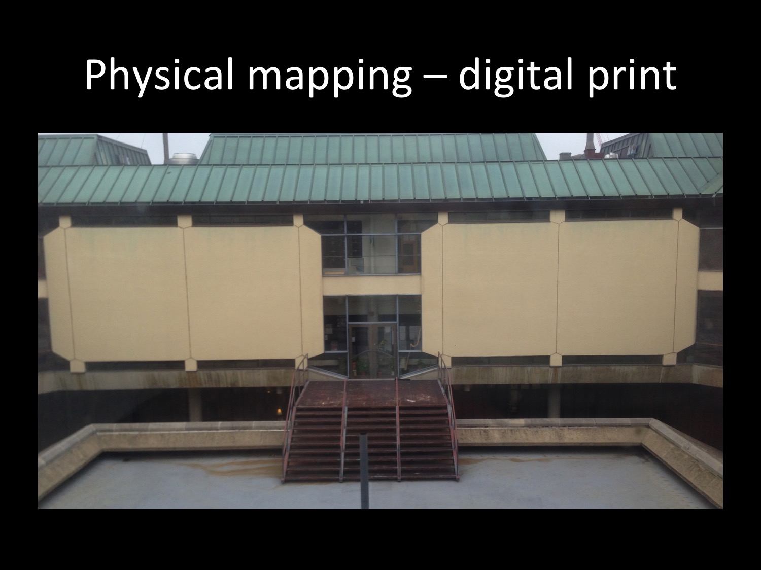
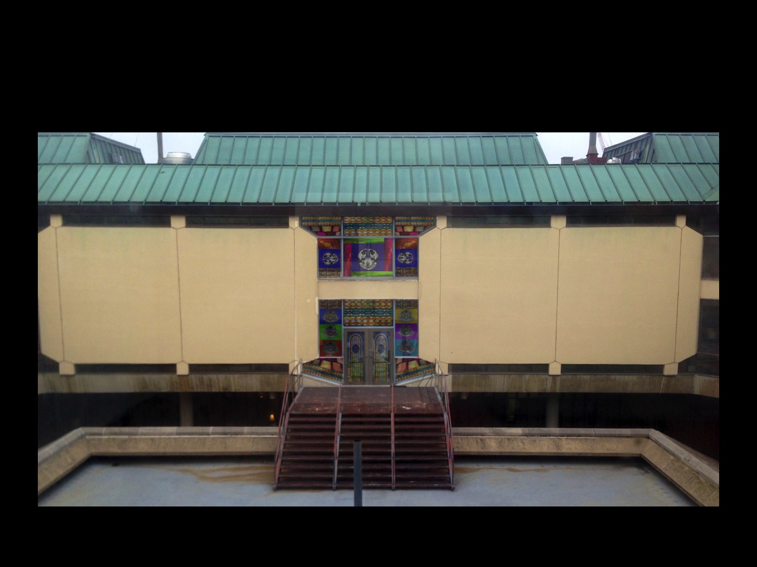
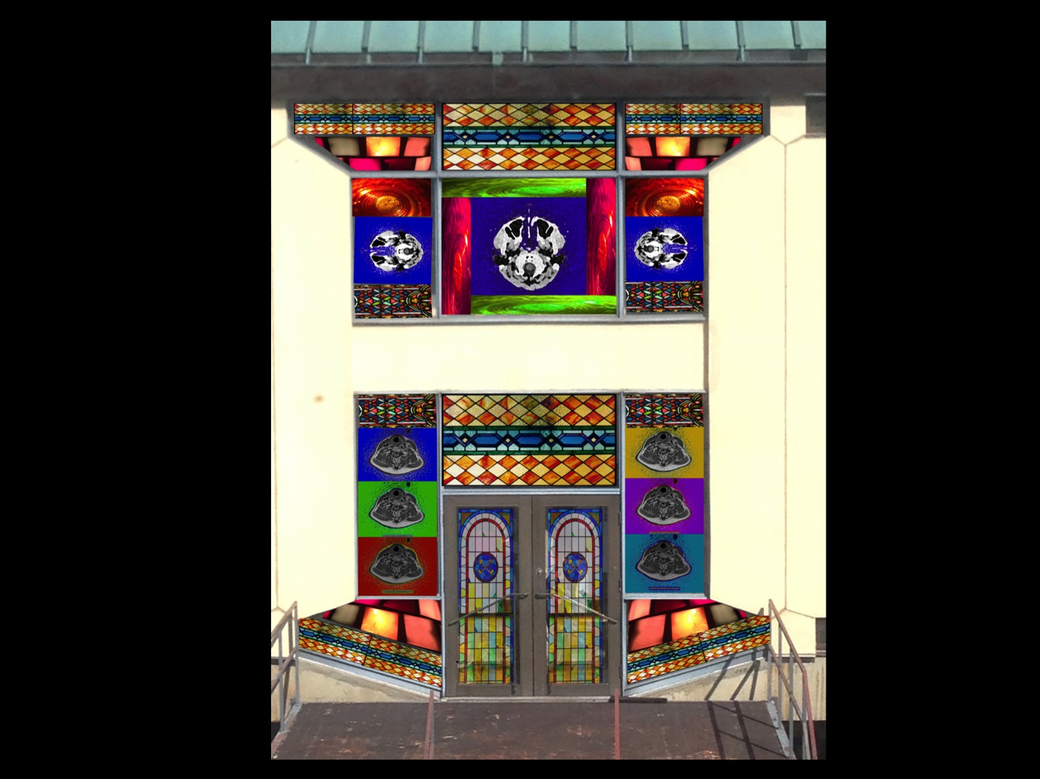
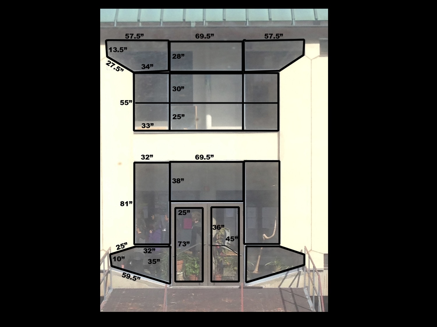
I am in mid of making glass mapping installation. There are totally 13 window panels in the physical architecture covering 6th and 7th floor of Humanities Building. I made the images following a narrative style in Medieval Gothic period, which scenes were typically designed to be read from the bottom of the stain glass window. In my research, I discovered there are not a standard code on which route the scenes flow from the bottom. Indeed, the flow of narrative varies. It can be a zigzag, from left to right proceeds upwards (or visa verses), or flow like a water fountain, or a combination of the above. The artisans had designed the narrative flow mainly in terms of the nature content and complexity of story and sub-story.

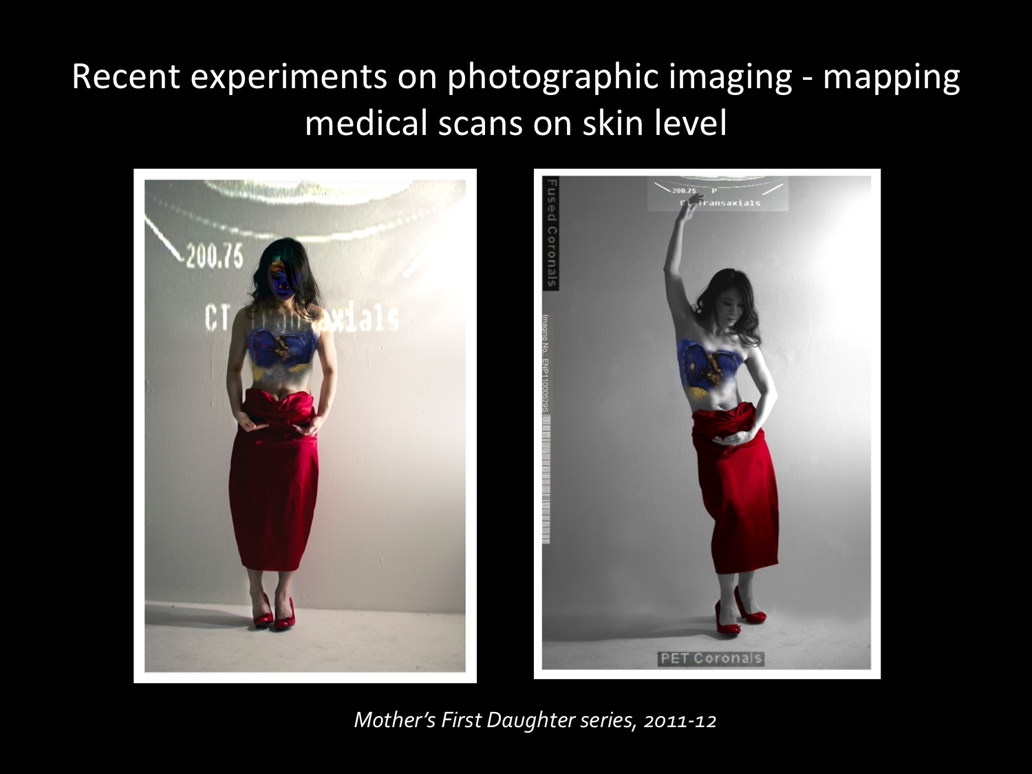
I took on this findings to start my narrative design at the bottom part. The bottom level is an genealogy of my in a perspective of family medical history. Biological and medical chemistry elements were sub-texts, serve as symbolism of my own medical body.

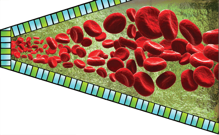
Panel 1 – red blood cells thrust across the space

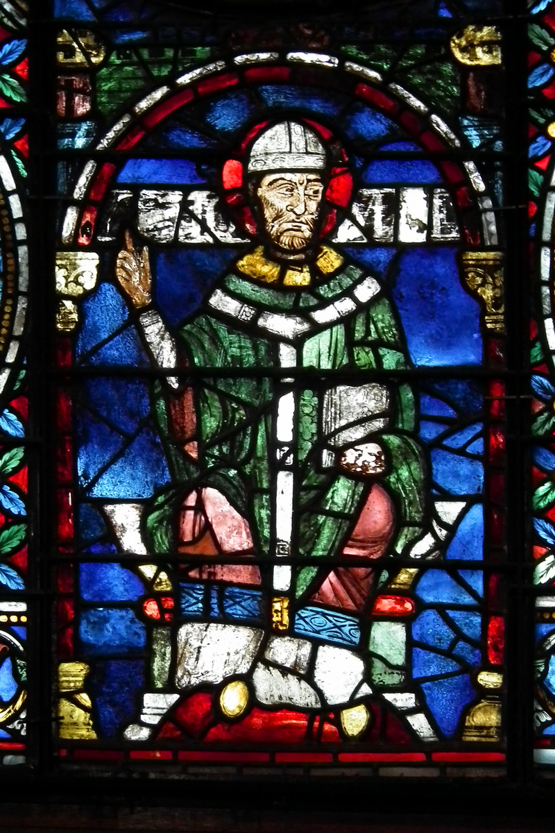
Panel 2 – Bottom part indicates my Mother’s medical condition: Red cancer cells form diagonal frames, Breast cancer MRI, chemical modules of chemotherapy. In upper part, there is a main character figure indicating he is a doctor or medical professional.

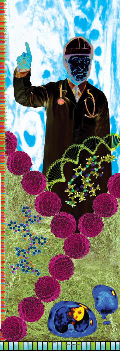
The image of this figure appears fit into a classic “medical authority” – western male in doctors gown with shirt and tie underneath. He has a stethoscope across his shoulders, while he points his right finger upwards. This is a gesture of saying something, or telling something. In fact, this image is an appropriation of the stain glass image of Archbishop Tomas Becket (21 December c. 1118  – 29 December 1170) of  Canterbury Church in London. I want to inject Becket ‘s miracle legend into a set of metaphor about healing, religious power and people beliefs in miracles.

Related Link:

https://en.wikipedia.org/wiki/Thomas_Becket

I decided to continue playing with forces this week before moving on to the next chapter. Two other types of force simulations that I hadn’t explored were fluid resistance and object to object attraction. I created two compositions which can be seen here and here.

Each composition contains two classes and there was an issue which led me to have to recode one function from one class into another for the simulation to work. With the algorithm having two classes that need to act together, there need to be functions in either one of the classes that reference an object of the other class.

I wanted to add a region to the sketch where the particles would experience a fluid resistance akin to falling into water or an air pocket. There are two key aspects of adding selective fluid resistance to our simulation. First, there needs to be a function that detects a “collision” with the region and returns a boolean, which would be used to activate a certain behavior. The behavior we are wanting to activate when a particle collides with our region is the initiation of a new force to be added. So secondly, there needs to be a function that defines the force to be experienced. When I was adding fluid resistance functionality to my particle string, I opted to add this functionality to the Particle class rather than to the Liquid class. But it didn’t work. If it did, we would expect the smaller particles (which are assigned a smaller mass), to experience greater attenuation of speed as they go down.

Fluid Resistance functionality added to Particle class did not work’

Main Draw program code that gives evaluates whether a particle is inside the fluid region and if so, adds a force to the particle

Anyways, as soon as I incorporated the functionality into the Liquid class, the region was producing a force on the particles as expected.

Separation of particles due to fluid resistance

I am still unsure why my first attempt was not successful because technically everything should have worked. I was referencing the liquid class.

When coding for the attractor, it should technically be possible to produce a simulation with the particle class becoming attracted to the attractor rather than the attractor attracting the particles. The technical difference lies in which of the classes references the other. But since I didn’t have much luck with particles referencing in their class the object that would produce their forces, I went with the second scenario of having the force entity reference the particles.

This week I will cover Chapter 3: Oscillations and produce attractions between each particle.

See you soon.

This week’s topic was Forces and simulating forces in the Processing environment. The main content from now on will come from “The Nature of Code” as I have finally learned all of the basics to the language and I am finally making particle simulations. The downside is that now things are more complex and even though I was able to swift through a lot of the preliminary content, I am finding myself getting stuck a lot more.

In any case, let me give a brief run on the forces that we looked at in Chapter 2 of “The Nature of Code”. We now have the PVector class that we know how to use so we can begin to use Physics to model motion under acceleration. Since Processing’s basic unit is a pixel, the distance units become pixels and the velocity units become pixels per frame. The chapter gave me a brief intro into classical mechanics with Newton’s Laws. We looked at gravitational force, friction forces and drags. But these end up being an approximation. The world we are simulating in Processing doesn’t really stand a chance against more sophisticated physics algorithms. Instead, what we should strive to do with simulations is to make them “look” like they are something.

For this weeks project I incorporated forces into the Particle String composition from week 7. This took me a long time to get right. Rather than use a force as described in the book, I decided to make up a force that would the particles stick to the sides of the window. The result feels like a viscous fluid splattering inside a box. Notice that if you keep the left mouse button pressed as you move your cursor around, the particles create a string, almost like a snake that follows the cursor. This was accomplished by incrementally setting up the the limiting velocity for each particle. The composition can be seen here.

Project progress:

Physical Image mapping – Architectural installation

Site: 6/F and 7/F glass windows, Humanities Building, UW-Madison

Initial image mock up (graphic content shown are sample only):

Close-up of Initial image mock up (graphic content shown are sample only):

Measurements of physical architecture:

Initial project ideas:

Long-term research interest direction diagram:

BACK-END DEVELOPMENT

We are continuing to structure the backend of our system and map out user (and data) flows and are starting to implement the services together as a cohesive, scalable system. We are looking to hire a student hourly to help the backend development move quickly.

FRONT-END DEVELOPMENT

We continue to brainstorm and implement different interfaces. We are now looking at these ideas under more scrutiny with certain UI/UX principles in mind. Development in Unity has been slowed down as we are transitioning from the IoT Lab to our new office at SoHE, but will pick up in the coming weeks.

BUSINESS DEVELOPMENT

As we refine our high level product and go to market solutions, our first phase continues with advancing our efforts in connecting with developers. Through meetings and conferences we have established initial contact with a lot of the developers that we want to be a part of our ecosystem. The next step is to follow up with those initial contacts and continue expanding our network of developers. We’ve come up an email draft to initiate conference calls to keep the developers in our network up to speed on what we’re working on so they can quickly be brought into test our alpha and beta builds.

This week I covered Chapters 13 and 14 of Learning Processing. I did fall a little behind schedule so I am posting this a little late. According to the syllabus, I was also supposed to cover the Chapter on Vectors in “The Nature of Code” but I already covered that two weeks ago.

A lot of what was covered last week in the Introduction to “The Nature of Code” is dealt with in Chapter 13 entitled Mathematics. I did not touch some of the content in more detail so I will do that now.

Last week, we delved a little on randomness and how randomness as modeled using some mathematical algorithms is not entirely random. Over time, if the random() function in Processing is run for a long enough time, a certain pattern would emerge. This means that random() produces a “uniform” distribution of numbers. When it comes to coding a natural-looking simulation, most so than often we will want to create a non-uniform distribution. In other words, we would like to create some numbers that tend to be favored over others. Dr. Shiffman offers two strategies to manipulate our random() into behaving more naturally by making use of probabilities in our code. The first one is to create an array where some numbers are more frequent than others and invoke a conditional that would do a block of code if one of these more frequent numbers is chosen by random(), type casted as integer. The second option is to let random() choose a number between 0 and 1 and create a series of conditionals that test for whether the random number is below or above a certain range, i.e. if n is between 0.00 and 0.60, the outcome under this conditional would have 60% chance of happening.

Another important concept is the alternative use of the noise(), which implements the Perlin noise algorithm, because in contrast to random(), the produced numbers constitute a “smoother” sequence. But noise() operates a little different because its argument is time. Noise() always outputs a number between 0 and 1. And we must scale it, ideally according to the dimensions of our sketch window.

After the discussion on randomness and noise, Chapter 13 reviews a few key ideas on trigonometry and oscillation and how sines and cosines are very well tailored for making elegant animations because they are such well behaved functions. Even though, Processing uses a cartesian coordinate system, we can easily use polar coordinate equations and convert them to cartesian when drawing shapes. Here is my solution to an exercise for creating a spiral in Processing. The idea is to draw a circle following the path traced by the spiral:

Spiral drawn with a circle

The final topic we covered was Recursion and the coding of recursive functions, that is, functions that call themselves in their definition. Here is a solution to a recursive design problem in the book involving circles:

Recursive Circles

Chapter 14 mainly talks about the use of transformations to translate, rotate, and scale our sketches as well as the use of transformation matrices in Processing. If you reference my solution to Exercise 13.5, you’ll see that I had to make an offset of width/2 for the x coordinate of the center of each circle and height/2 for the y coordinate since our parametric equation for the spiral produces the spiral around (0,0) and in the Processing coordinate system our (0,0) is at the top left corner. A transformation function like translate() allows us to change the center of our coordinate system and put it whereever we like, offsetting the geometry on the canvas accordingly. Similarly rotate() allows us to rotate our coordinate system and make our composition rotate about an angle. Since functions like translate() and rotate() are additive and affect any shape that is drawn after they are called, Processing provides us with means to separate, save and restore transformation matrices so that we can tailor our transformations selectively as we like. Al

I didn’t have time to incorporate Perlin noise() or beginShape into a particle system like the project for this week calls for. But I wanted to implement the use of pushMatrix and popMatrix into a sketch so I did the following composition

See you next week.

This week I covered Chapter 10 of “Learning Processing” and the introduction chapter to “The Nature of Code”. Chapters 11 and 12 were skimmed. These just described how to install libraries for Processing to expand its functionality and debugging. But Chapter 10 and the Intro to “The Nature of Code” contained the more important information.

Chapter 10 felt more like a recap to unify all that we have learned so far before moving on to bigger things. As such, it simply presented a concrete framework to use as a guideline when developing algorithms in Processing. It goes as follows:

1 – Come up with an idea

2 – Break the idea into smaller parts

3- Work out the algorithm for each part

4- Write the code for each part

5- Work out the algorithm for all parts together

6- Integrate the code for all of the parts together

The way I would be using this framework in the development of autonomous agents and particle systems is to isolate each behavior and code that separately first, then integrate them in the final program. The author does this with a game in which each element of the game is written in a different class and the final game code combines all three classes together.

On to the Introduction of “The Nature of Code”…

In this section, we code our first autonomous agent using a Walker class. For exercise I.1 we are asked to code the behavior of an agent that has the tendency to move down and to the right. Here’s my solution and the pattern it produced.

First Basic Agent. Exercise I.1

Interestingly, if you let the script run for an hour, you get this very interesting textured canvas. This texture could actually be saved and edited in Photoshop to create a bump map or normal map for a material. It could simulate the roughness of a wooden surface.

Processing’s random number generator is one that produces a uniform distribution of numbers. If we want a non-uniform distribution of numbers, then we must combine randomness with probability, making it possible for some numbers to be picked more often than others, just like nature tends to favor certain values over others, i.e., in coding an evolutionary algorithm, one would need to make sure certain elements were selected more often than others according to the Darwinian thesis of “survival of the fittest”. Most properties of a natural entity , for example, a person’s height, are not uniformly distributed across a collection of those entities. There are more people of average height than there are people who are either really tall or really short. We can use the Random Class from Java to produce a random number with a normal distribution.

On to this week’s project… I had a little bit of a struggle with this one. I still haven’t documented my code but I will do that before the end of the week. This week’s project built upon last week’s and involved the creation of a tail for each of our particles. This amounted to devising a second particle system which would constitute the tail. The tail of each of the particles is essentially a trail of ellipses drawn together. In the code, the number of ellipses is given by tailLength and the separation of one ellipse from another is given by tailStep.

The composition can be played here

Something is not working right but I managed to at least have tails for each particle. I will take care of refining this for next week.

Thanks.