This week I covered Chapter 3 of “The Nature of Code”. The chapters keep getting  more and more in depth and the exercises more complicated. But I was able to finish two of the exercises and create a neat little artistic particle system using a trig function to define a boundary. You can see it here.

In the past we have covered motion and we borrow the same principles of motion simulation to model oscillation in the Processing environment. Before we had the following two key statements to make agents move:

location.add(velocity);

Now for oscillation we use:

angle.add(avelocity);

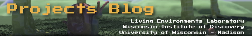
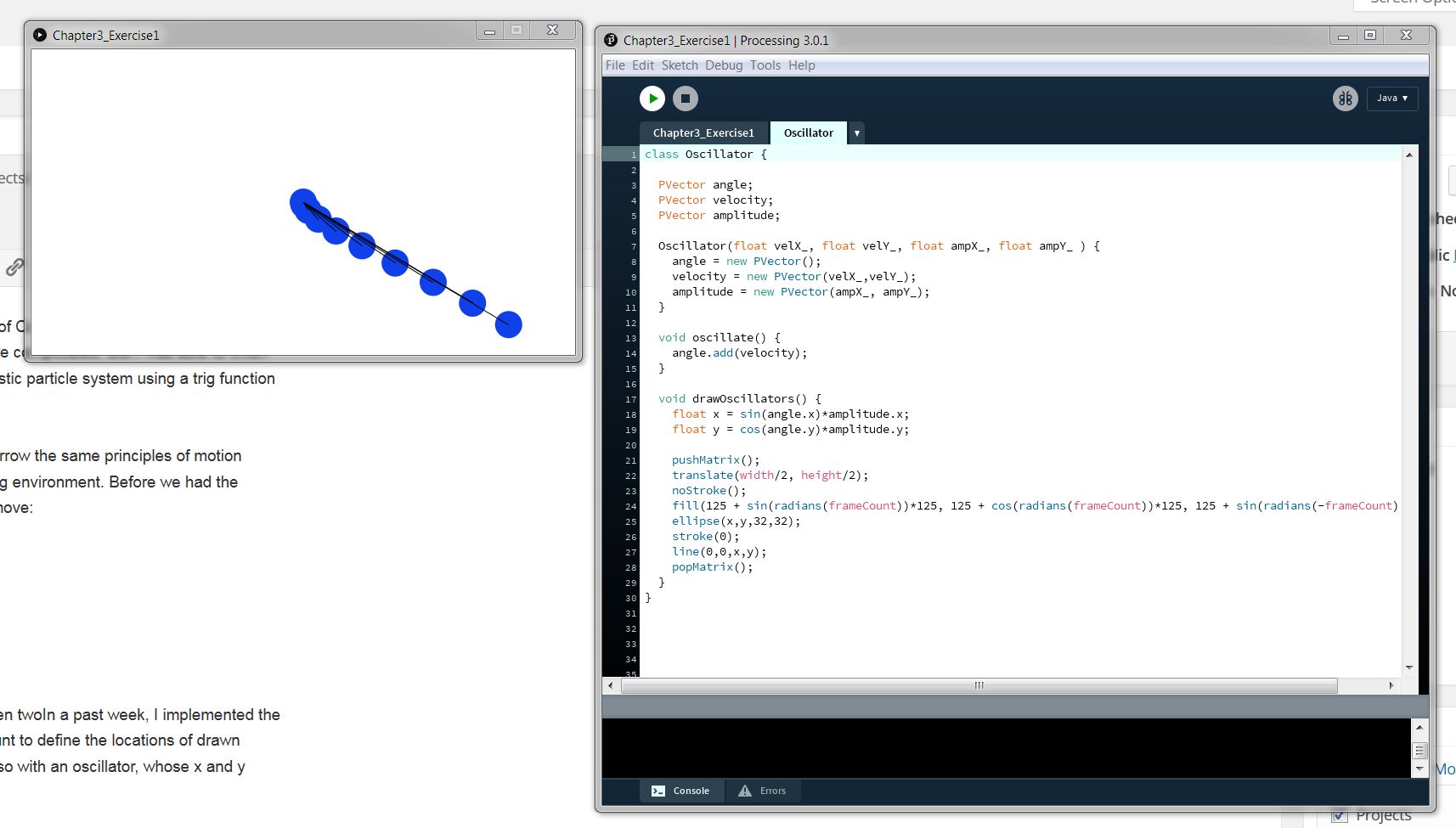
We know that both sin and cos oscillate between (-1,1). In a past week, I implemented the notion of using trig functions with the frameCount to define the locations of drawn elements. This is essentially what we will do also with an oscillator, whose x and y coordinates will be given by Amplitude * sin( some increasing angle) and Amplitude * cos (some increasing angle). The first exercise asked me to find a way to make a pattern out of an array of oscillators. I used trig functions to make initialize the velocities in a rhythmic pattern:

Oscillator class\

Initialization of Oscillators’ velocities with trig functions

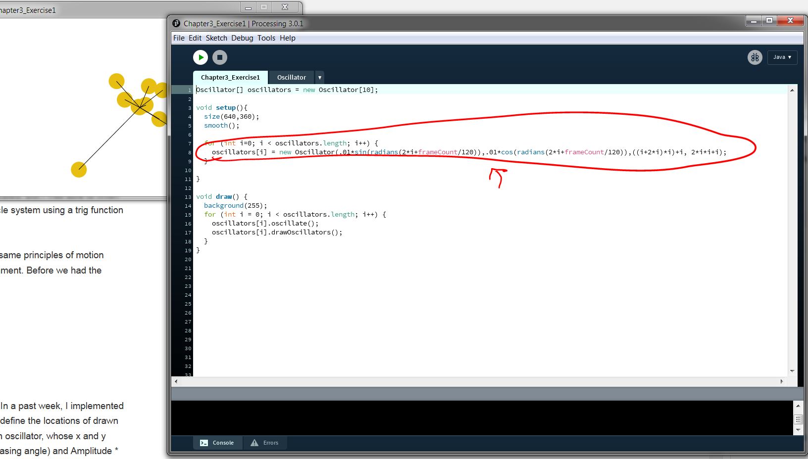
We also looked at waves. The exercise I did required me to encapsulate a wave into a class and create a pattern:

Wave Class and Pattern

This week I will be looking at Chapter 4 and hopefully conceive a colliding particle system.

See you soon.