This week covered Chapter 5 of “The Nature of Code” which introduces us to a very useful library for physics based simulations called Toxiclibs.

I am using Toxiclibs to create my final composition because it is great to produce compositions based on vector fields. However this chapter focused on Toxiclibs classes to simulate soft bodies. Toxiclibs contains it’s own set of particles package called VerletParticles, and  springs called VerletSprings. When you first begin a sketch using Toxiclibs you will have to include an import statement for a particular package to reference back to the methods and classes that you are going to use. The reference doc is very extensive and can be found here.

For the chapter, I completed the exercise that asked to develop a softbody cloth using a grid of particles connected by strings. This required once again, much like in the shatter example, the need to arrange particles in a grid separeted by a distance which would equal the rest distance of the spring. Below is a screenshot of the simulation:

Cloth Simulation

For this week’s composition, I decided to still continue with the particle systems and leave the use of toxiclibs for my final composition. I wanted to try something more geometrical and thought that I could come up with an evolving polygon by having particles connect to each other as they moved abt the screen space. In the future, an export of these lines to a CAD software can be incorporated into the application such that the 2D forms could be used as the starting basis of a floor plan. My sketch can be played here.

I haven’t gotten a chance to talk about Polymorphism and Inheritance from Chapter 4 yet so I wanted to make a post about them.

We have seen how coding particle systems becomes a lot more intuitive when done in an object – oriented way by creating classes and defining arrays of objects of those classes. In more complicated scenarios, we may want to have more than one type of particle or agent with specific functions associated with it. Even then, it is very likely that each class will still have a lot of the same properties; since they are particles, their constructors will all have location vectors, velocity vectors and acceleration vectors. Moreover, their functions for describing motion may be the same. So it would seem like a good idea if we could re use the code in some way. Inheritance allows us to do this very easily by extending the properties of another class. So a class that inherits another class becomes a subclass of that class:

class Cat extends Animal {
  Cat() {
    super();
  }
  void meow() {
    println("MEOW!");
  }
}

This means that the cat inherits all of the properties and functions of the Animal. Using super() makes sure that the same initialized properties of the Animal(height, weight) are given to the cat. Also any functions of the animal, for example, eat(), sleep() are also now applicable to the cat. In addition to those functions, the cat object can have its own functions.

So what becomes of a cat object when it is extending another class? In cases where we are declaring arrays or arraylists, code specifies the type of objects that array will store,

ArrayList<Cat> kitty = new ArrayList<Cat>();

Polymorphism makes it possible to store subclasses of a class together as if they were the same type. So it is now perfectly valid to say

ArrayList<Animal> kitty = new ArrayList<Cat>();

With particles systems, this enables us to store all types of particles into one array as long as all the subclasses extend the same Particle class.

For this week’s project, I wanted to make sure that I was able to do particle system branched out into a particle class and a particlesystem subclass. This is a good way to start getting into the habit of coding a particle type and then a particle controller. First I did two exercises out of the chapter.

The first exercise asked for a movable rocket. This was basically an extension of Week 10 sketch of having a particle system moving while releasing particles.

Asteroid Exercise

The second exercise wanted a geometrical form to divide into smaller pieces or shatter. This amounted to using our regular Particle class and then having our ParticleSystem class arrange them in a grid. I wasn’t able to center it in the middle so I think my arrangement was off. When you clicked on the canvas, the particles began their kinematic method and started moving as if shattering.

Shatter Exercise

For this week’s script, I decided to do another particle system but this time incorporating oscillation kinematics, as covered in Chapter 3, to give the particles a more life-like appearance. The particle system was done following the style of using two classes, one for the particle and one for the particlesystem. You may see the script here. Originally I had planned to incorporate the collisions in this script but I ran out of time.

Finished it. Yes! The script for colliding particles can be seen here. More to come about inheritance and polymorphism tomorrow.

Unfortunately, Chapter 4, namely, Particle Systems will require another week to finish. That’s not so bad since after chapter 4, there are only 2 more chapters to finish this semester’s main learning curriculum. There are a few sections of Chapter 4 on inheritance and polymorphism that I did not get to cover because I ran out of time.

The sections I covered of Chapter 4 discussed the idea of not just having one particle class but rather having multiple classes communicating with one another to handle systems of systems of particles. The other topic covered was coding in lifespan for each particle so that the program did not bottleneck from continuing to draw all the particles emitted. The author introduced the arraylist class, though I had already been using it since Week 5 when I decided to jumpstart on composing particle systems. I was introduced to this more convenient form of an array in  brief look I had on Chapter 23 of “Learning Processing”. For particle systems, it is extremely convenient since it allows straightforward resizing of the array by adding and removing items. The regular array can also be resized but it is not as easy as just “arrayname.add” or “arrayname.remove”. As my weekly composition, I decided to do one of the exercises that required me to make a moving emitter. The sketch can be seen here.

I spent most of the week trying to tackle the problem of collision, something Prof. Ponto suggested. It actually turns out to be a little bit more complicated than I thought (lol). Prof. Schiffman actually dedicates an entire chapter, the next chapter I am supposed to cover, on the use of an external physics engine built for Java called Box2D for collisions. But he also says it is possible to tackle simple collisions without the need of an additional class library like Box2D. Anyways I feel I am getting close but I still don’t have a working composition for the collisions of multiple particles. But here’s what I got so far.

Okay so the basic pseudo algorithm we are looking to code is as follows:

Bounce Function

This week I covered Chapter 3 of “The Nature of Code”. The chapters keep getting  more and more in depth and the exercises more complicated. But I was able to finish two of the exercises and create a neat little artistic particle system using a trig function to define a boundary. You can see it here.

In the past we have covered motion and we borrow the same principles of motion simulation to model oscillation in the Processing environment. Before we had the following two key statements to make agents move:

location.add(velocity);

Now for oscillation we use:

angle.add(avelocity);

We know that both sin and cos oscillate between (-1,1). In a past week, I implemented the notion of using trig functions with the frameCount to define the locations of drawn elements. This is essentially what we will do also with an oscillator, whose x and y coordinates will be given by Amplitude * sin( some increasing angle) and Amplitude * cos (some increasing angle). The first exercise asked me to find a way to make a pattern out of an array of oscillators. I used trig functions to make initialize the velocities in a rhythmic pattern:

Oscillator class\

Initialization of Oscillators’ velocities with trig functions

We also looked at waves. The exercise I did required me to encapsulate a wave into a class and create a pattern:

Wave Class and Pattern

This week I will be looking at Chapter 4 and hopefully conceive a colliding particle system.

See you soon.

I decided to continue playing with forces this week before moving on to the next chapter. Two other types of force simulations that I hadn’t explored were fluid resistance and object to object attraction. I created two compositions which can be seen here and here.

Each composition contains two classes and there was an issue which led me to have to recode one function from one class into another for the simulation to work. With the algorithm having two classes that need to act together, there need to be functions in either one of the classes that reference an object of the other class.

I wanted to add a region to the sketch where the particles would experience a fluid resistance akin to falling into water or an air pocket. There are two key aspects of adding selective fluid resistance to our simulation. First, there needs to be a function that detects a “collision” with the region and returns a boolean, which would be used to activate a certain behavior. The behavior we are wanting to activate when a particle collides with our region is the initiation of a new force to be added. So secondly, there needs to be a function that defines the force to be experienced. When I was adding fluid resistance functionality to my particle string, I opted to add this functionality to the Particle class rather than to the Liquid class. But it didn’t work. If it did, we would expect the smaller particles (which are assigned a smaller mass), to experience greater attenuation of speed as they go down.

Fluid Resistance functionality added to Particle class did not work’

Main Draw program code that gives evaluates whether a particle is inside the fluid region and if so, adds a force to the particle

Anyways, as soon as I incorporated the functionality into the Liquid class, the region was producing a force on the particles as expected.

Separation of particles due to fluid resistance

I am still unsure why my first attempt was not successful because technically everything should have worked. I was referencing the liquid class.

When coding for the attractor, it should technically be possible to produce a simulation with the particle class becoming attracted to the attractor rather than the attractor attracting the particles. The technical difference lies in which of the classes references the other. But since I didn’t have much luck with particles referencing in their class the object that would produce their forces, I went with the second scenario of having the force entity reference the particles.

This week I will cover Chapter 3: Oscillations and produce attractions between each particle.

See you soon.

This week’s topic was Forces and simulating forces in the Processing environment. The main content from now on will come from “The Nature of Code” as I have finally learned all of the basics to the language and I am finally making particle simulations. The downside is that now things are more complex and even though I was able to swift through a lot of the preliminary content, I am finding myself getting stuck a lot more.

In any case, let me give a brief run on the forces that we looked at in Chapter 2 of “The Nature of Code”. We now have the PVector class that we know how to use so we can begin to use Physics to model motion under acceleration. Since Processing’s basic unit is a pixel, the distance units become pixels and the velocity units become pixels per frame. The chapter gave me a brief intro into classical mechanics with Newton’s Laws. We looked at gravitational force, friction forces and drags. But these end up being an approximation. The world we are simulating in Processing doesn’t really stand a chance against more sophisticated physics algorithms. Instead, what we should strive to do with simulations is to make them “look” like they are something.

For this weeks project I incorporated forces into the Particle String composition from week 7. This took me a long time to get right. Rather than use a force as described in the book, I decided to make up a force that would the particles stick to the sides of the window. The result feels like a viscous fluid splattering inside a box. Notice that if you keep the left mouse button pressed as you move your cursor around, the particles create a string, almost like a snake that follows the cursor. This was accomplished by incrementally setting up the the limiting velocity for each particle. The composition can be seen here.

This week I covered Chapters 13 and 14 of Learning Processing. I did fall a little behind schedule so I am posting this a little late. According to the syllabus, I was also supposed to cover the Chapter on Vectors in “The Nature of Code” but I already covered that two weeks ago.

A lot of what was covered last week in the Introduction to “The Nature of Code” is dealt with in Chapter 13 entitled Mathematics. I did not touch some of the content in more detail so I will do that now.

Last week, we delved a little on randomness and how randomness as modeled using some mathematical algorithms is not entirely random. Over time, if the random() function in Processing is run for a long enough time, a certain pattern would emerge. This means that random() produces a “uniform” distribution of numbers. When it comes to coding a natural-looking simulation, most so than often we will want to create a non-uniform distribution. In other words, we would like to create some numbers that tend to be favored over others. Dr. Shiffman offers two strategies to manipulate our random() into behaving more naturally by making use of probabilities in our code. The first one is to create an array where some numbers are more frequent than others and invoke a conditional that would do a block of code if one of these more frequent numbers is chosen by random(), type casted as integer. The second option is to let random() choose a number between 0 and 1 and create a series of conditionals that test for whether the random number is below or above a certain range, i.e. if n is between 0.00 and 0.60, the outcome under this conditional would have 60% chance of happening.

Another important concept is the alternative use of the noise(), which implements the Perlin noise algorithm, because in contrast to random(), the produced numbers constitute a “smoother” sequence. But noise() operates a little different because its argument is time. Noise() always outputs a number between 0 and 1. And we must scale it, ideally according to the dimensions of our sketch window.

After the discussion on randomness and noise, Chapter 13 reviews a few key ideas on trigonometry and oscillation and how sines and cosines are very well tailored for making elegant animations because they are such well behaved functions. Even though, Processing uses a cartesian coordinate system, we can easily use polar coordinate equations and convert them to cartesian when drawing shapes. Here is my solution to an exercise for creating a spiral in Processing. The idea is to draw a circle following the path traced by the spiral:

Spiral drawn with a circle

The final topic we covered was Recursion and the coding of recursive functions, that is, functions that call themselves in their definition. Here is a solution to a recursive design problem in the book involving circles:

Recursive Circles

Chapter 14 mainly talks about the use of transformations to translate, rotate, and scale our sketches as well as the use of transformation matrices in Processing. If you reference my solution to Exercise 13.5, you’ll see that I had to make an offset of width/2 for the x coordinate of the center of each circle and height/2 for the y coordinate since our parametric equation for the spiral produces the spiral around (0,0) and in the Processing coordinate system our (0,0) is at the top left corner. A transformation function like translate() allows us to change the center of our coordinate system and put it whereever we like, offsetting the geometry on the canvas accordingly. Similarly rotate() allows us to rotate our coordinate system and make our composition rotate about an angle. Since functions like translate() and rotate() are additive and affect any shape that is drawn after they are called, Processing provides us with means to separate, save and restore transformation matrices so that we can tailor our transformations selectively as we like. Al

I didn’t have time to incorporate Perlin noise() or beginShape into a particle system like the project for this week calls for. But I wanted to implement the use of pushMatrix and popMatrix into a sketch so I did the following composition

See you next week.

This week I covered Chapter 10 of “Learning Processing” and the introduction chapter to “The Nature of Code”. Chapters 11 and 12 were skimmed. These just described how to install libraries for Processing to expand its functionality and debugging. But Chapter 10 and the Intro to “The Nature of Code” contained the more important information.

Chapter 10 felt more like a recap to unify all that we have learned so far before moving on to bigger things. As such, it simply presented a concrete framework to use as a guideline when developing algorithms in Processing. It goes as follows:

1 – Come up with an idea

2 – Break the idea into smaller parts

3- Work out the algorithm for each part

4- Write the code for each part

5- Work out the algorithm for all parts together

6- Integrate the code for all of the parts together

The way I would be using this framework in the development of autonomous agents and particle systems is to isolate each behavior and code that separately first, then integrate them in the final program. The author does this with a game in which each element of the game is written in a different class and the final game code combines all three classes together.

On to the Introduction of “The Nature of Code”…

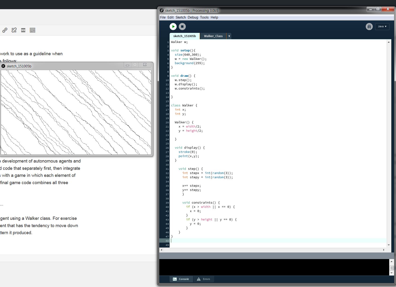
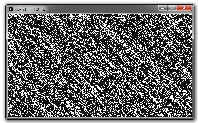
In this section, we code our first autonomous agent using a Walker class. For exercise I.1 we are asked to code the behavior of an agent that has the tendency to move down and to the right. Here’s my solution and the pattern it produced.

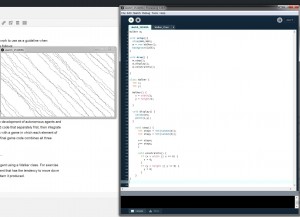
First Basic Agent. Exercise I.1

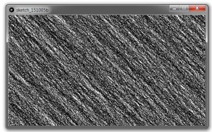
Interestingly, if you let the script run for an hour, you get this very interesting textured canvas. This texture could actually be saved and edited in Photoshop to create a bump map or normal map for a material. It could simulate the roughness of a wooden surface.

Processing’s random number generator is one that produces a uniform distribution of numbers. If we want a non-uniform distribution of numbers, then we must combine randomness with probability, making it possible for some numbers to be picked more often than others, just like nature tends to favor certain values over others, i.e., in coding an evolutionary algorithm, one would need to make sure certain elements were selected more often than others according to the Darwinian thesis of “survival of the fittest”. Most properties of a natural entity , for example, a person’s height, are not uniformly distributed across a collection of those entities. There are more people of average height than there are people who are either really tall or really short. We can use the Random Class from Java to produce a random number with a normal distribution.

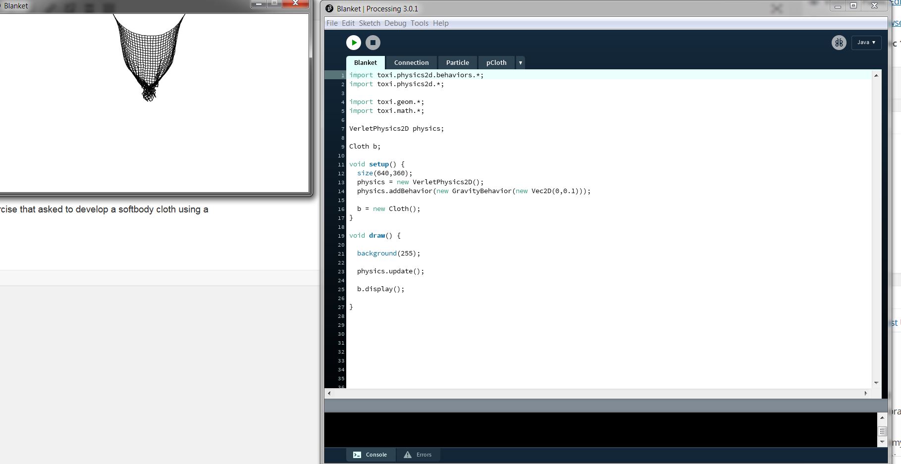
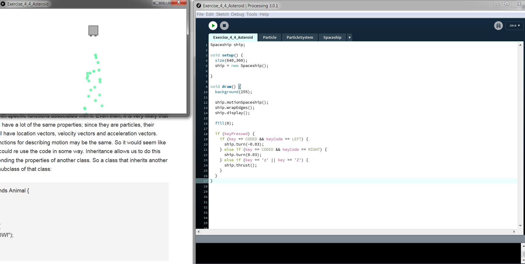
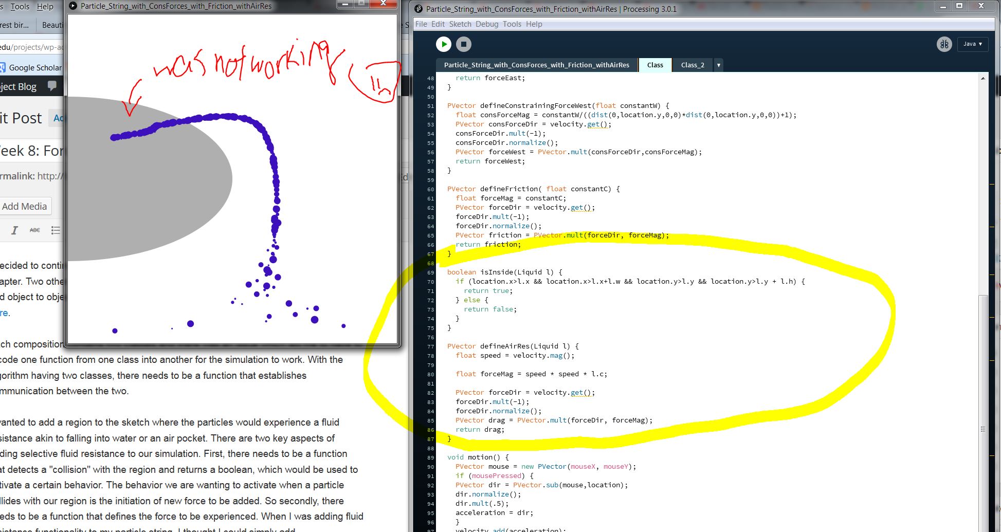
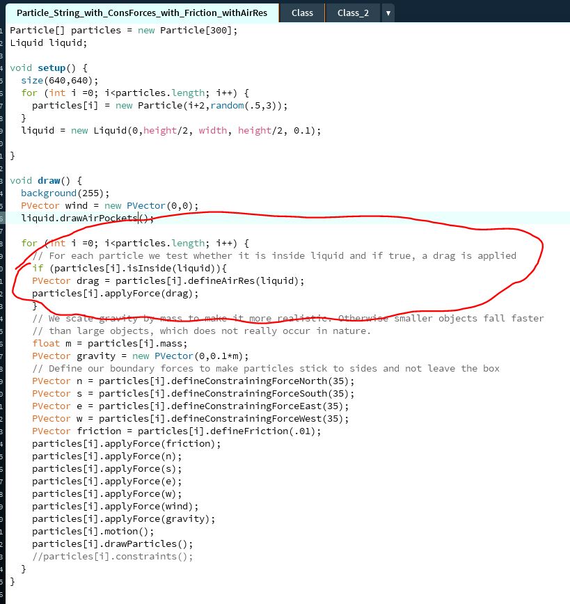
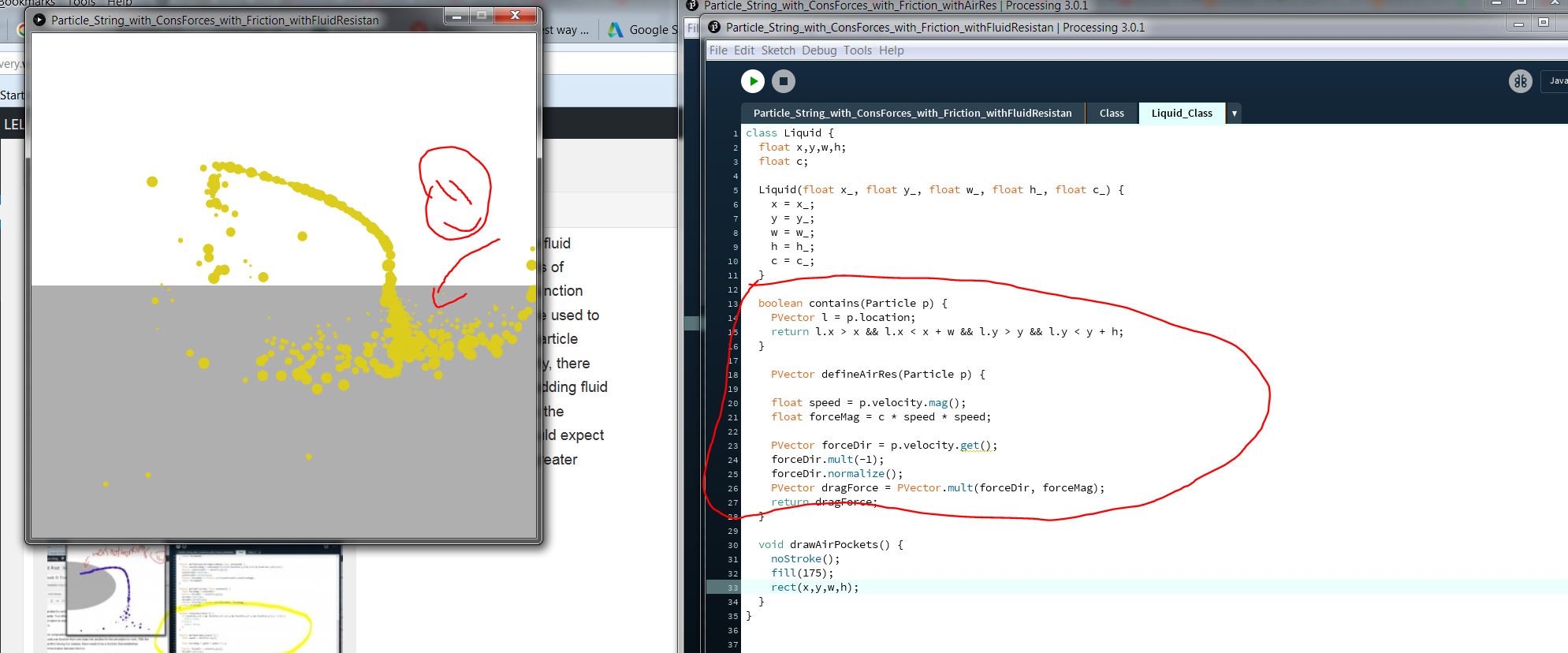
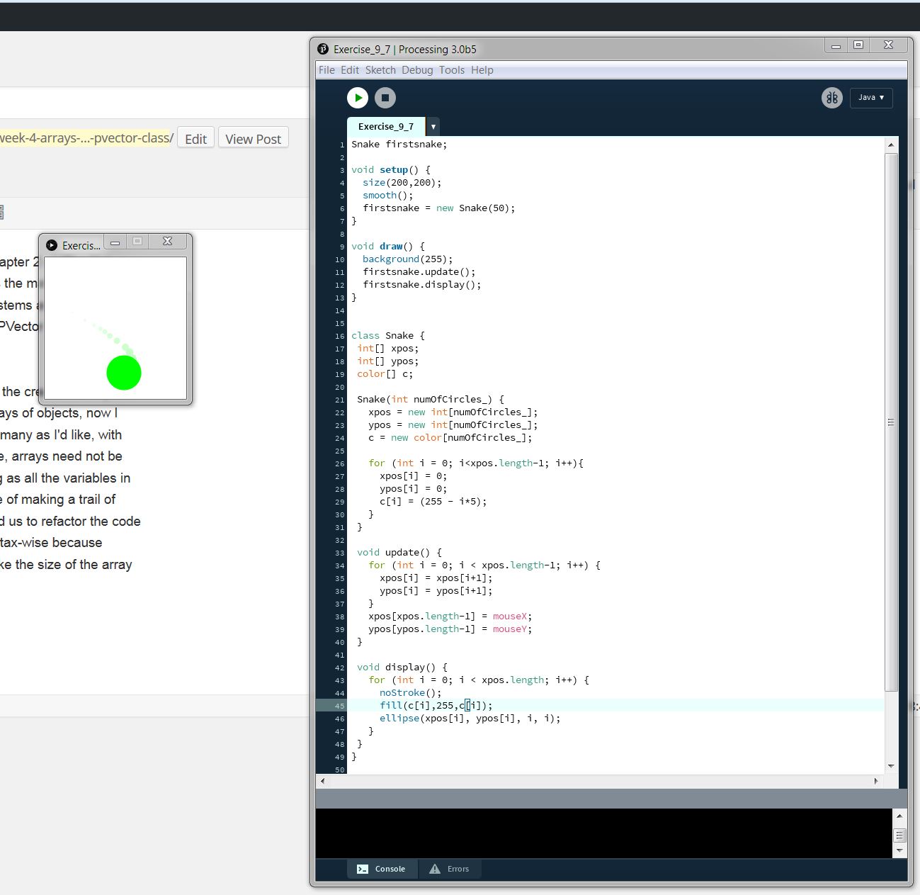
On to this week’s project… I had a little bit of a struggle with this one. I still haven’t documented my code but I will do that before the end of the week. This week’s project built upon last week’s and involved the creation of a tail for each of our particles. This amounted to devising a second particle system which would constitute the tail. The tail of each of the particles is essentially a trail of ellipses drawn together. In the code, the number of ellipses is given by tailLength and the separation of one ellipse from another is given by tailStep.

The composition can be played here

Something is not working right but I managed to at least have tails for each particle. I will take care of refining this for next week.

Thanks.

This week I studied Chapter 9 of “Learning Processing”, and Chapter 2 of “The Nature of Code”. This is a little different than what I had originally set as the material for Week 4 but I really wanted to start dealing with vectors and particle systems and it seemed like a good idea to mix the material dealing with Arrays and the PVector class together since they are both complementary to one another.

Last week I was introduced to object-oriented programming and the creation of objects to make our Processing more flexible and modular. By using arrays of objects, now I can automate the creation and animation of multiple objects, as many as I’d like, with the use of for loops, dot notation and array operations. Of course, arrays need not be just objects, they are free to contain any type of variable, as long as all the variables in the array are of the same type. The book presented the example of making a trail of ellipses follow a mouse cursor. As the exercise, the author asked us to refactor the code using an object-oriented approach. This was a little bit tricky syntax-wise because arrays needed to be declared and initialized and I wanted to make the size of the array an argument that could easily be changed. Here is my solution:

Solution to Exercise

On to PVectors… They are a class in Processing made to help model motion and physics. We know abt vectors. Velocity, Acceleration and position are all vector quantities. You can do algebra with vectors, you can do calculus with vectors. Particle systems will often operate under certain motion simulations and this is why it becomes necessary to make particles use PVectors. Otherwise we would need to have variables of motion for x, y, and z separately.

Owing to the knowledge I gained from Chapter 2, I was able to code a basic particle system that responds to mouse presses making each particle’s acceleration be toward the cursor each time the mouse is pressed. This is my project for the week and you may interact with the composition by clicking here. Next week, I will add a number of enhancements including trails and more realistic accelerations by including forces and dampening.

See you next week.